pacman::p_load(sf, spdep, tmap, tidyverse, knitr, GWmodel)In Class Exercise 5
1. Overview
2. Importing the Packages
In this in class exercise, we will be using the following packages:
3 Data Wrangling
3.1 Import shapefile into r environment
The code chunk below uses st_read() of sf package to import Hunan shapefile into R. The imported shapefile will be simple features Object of sf.
hunan <- st_read(dsn = "data/geospatial",
                 layer = "Hunan")
Reading layer `Hunan' from data source
`/Users/georgiaxng/georgiaxng/is415-handson/In-class_Ex/In-Class_Ex05/data/geospatial'
using driver `ESRI Shapefile'
Simple feature collection with 88 features and 7 fields
Geometry type: POLYGON
Dimension: XY
Bounding box: xmin: 108.7831 ymin: 24.6342 xmax: 114.2544 ymax: 30.12812
Geodetic CRS: WGS 843.2 Import csv file into r environment
Next, we will import Hunan_2012.csv into R by using read_csv() of readr package. The output is R dataframe class.
hunan2012 <- read_csv("data/aspatial/Hunan_2012.csv")3.3 Performing relational join
The code chunk below will be used to update the attribute table of hunan’s SpatialPolygonsDataFrame with the attribute fields of hunan2012 dataframe. This is performed by using left_join() of dplyr package.
hunan_sf <- left_join(hunan,hunan2012)%>%
  select(1:3, 7, 15, 16, 31,32)
Saving the output into a output file so that R studio will no longer need to waste time on the previous step.
write_rds(hunan_sf, "data/rds/hunan_sf.rds")Reading the data.
3.4 Converting to SpatialPolygonDataFrame
Note
GWmodel is built around the older sp and not sf formats for handling spatial data in R.
hunan_sp <- hunan_sf %>% as_Spatial()4 Geographically Weighted Summary Statistics with adaptive bandwidth
4.1 Determine Adaptive Bandwidth
4.1.1 AIC
bw_AIC <- bw.gwr(GDPPC ~ 1,
                 data = hunan_sp,
                 approach = "AIC",
                 adaptive = TRUE,
                 kernel = "bisquare",
                 longlat = T)
Adaptive bandwidth (number of nearest neighbours): 62 AICc value: 1923.156
Adaptive bandwidth (number of nearest neighbours): 46 AICc value: 1920.469
Adaptive bandwidth (number of nearest neighbours): 36 AICc value: 1917.324
Adaptive bandwidth (number of nearest neighbours): 29 AICc value: 1916.661
Adaptive bandwidth (number of nearest neighbours): 26 AICc value: 1914.897
Adaptive bandwidth (number of nearest neighbours): 22 AICc value: 1914.045
Adaptive bandwidth (number of nearest neighbours): 22 AICc value: 1914.045 Good thing with GWmodel is that automatically determines the bandwidth for you
Note
Unit of measurement for bandwidth value shown here is in kilometres.
4.1.2 Cross-validation
bw_AIC <- bw.gwr(GDPPC ~ 1,
                 data = hunan_sp,
                 approach = "CV",
                 adaptive = TRUE,
                 kernel = "bisquare",
                 longlat = T)
Adaptive bandwidth: 62 CV score: 15515442343
Adaptive bandwidth: 46 CV score: 14937956887
Adaptive bandwidth: 36 CV score: 14408561608
Adaptive bandwidth: 29 CV score: 14198527496
Adaptive bandwidth: 26 CV score: 13898800611
Adaptive bandwidth: 22 CV score: 13662299974
Adaptive bandwidth: 22 CV score: 13662299974 Identical to AIC, same number of results generated.
4.2 Determine Fixed Bandwidth
4.2.1 AIC
bw_AIC <- bw.gwr(GDPPC ~ 1,
data = hunan_sp,
approach = "AIC",
kernel = "bisquare",
adaptive = FALSE,
longlat = T)Fixed bandwidth: 357.4897 AICc value: 1927.631
Fixed bandwidth: 220.985 AICc value: 1921.547
Fixed bandwidth: 136.6204 AICc value: 1919.993
Fixed bandwidth: 84.48025 AICc value: 1940.603
Fixed bandwidth: 168.8448 AICc value: 1919.457
Fixed bandwidth: 188.7606 AICc value: 1920.007
Fixed bandwidth: 156.5362 AICc value: 1919.41
Fixed bandwidth: 148.929 AICc value: 1919.527
Fixed bandwidth: 161.2377 AICc value: 1919.392
Fixed bandwidth: 164.1433 AICc value: 1919.403
Fixed bandwidth: 159.4419 AICc value: 1919.393
Fixed bandwidth: 162.3475 AICc value: 1919.394
Fixed bandwidth: 160.5517 AICc value: 1919.391 4.2.2 Cross Validation
bw_AIC <- bw.gwr(GDPPC ~ 1,
data = hunan_sp,
approach = "CV",
kernel = "bisquare",
adaptive = FALSE,
longlat = T)Fixed bandwidth: 357.4897 CV score: 16265191728
Fixed bandwidth: 220.985 CV score: 14954930931
Fixed bandwidth: 136.6204 CV score: 14134185837
Fixed bandwidth: 84.48025 CV score: 13693362460
Fixed bandwidth: 52.25585 CV score: Inf
Fixed bandwidth: 104.396 CV score: 13891052305
Fixed bandwidth: 72.17162 CV score: 13577893677
Fixed bandwidth: 64.56447 CV score: 14681160609
Fixed bandwidth: 76.8731 CV score: 13444716890
Fixed bandwidth: 79.77877 CV score: 13503296834
Fixed bandwidth: 75.07729 CV score: 13452450771
Fixed bandwidth: 77.98296 CV score: 13457916138
Fixed bandwidth: 76.18716 CV score: 13442911302
Fixed bandwidth: 75.76323 CV score: 13444600639
Fixed bandwidth: 76.44916 CV score: 13442994078
Fixed bandwidth: 76.02523 CV score: 13443285248
Fixed bandwidth: 76.28724 CV score: 13442844774
Fixed bandwidth: 76.34909 CV score: 13442864995
Fixed bandwidth: 76.24901 CV score: 13442855596
Fixed bandwidth: 76.31086 CV score: 13442847019
Fixed bandwidth: 76.27264 CV score: 13442846793
Fixed bandwidth: 76.29626 CV score: 13442844829
Fixed bandwidth: 76.28166 CV score: 13442845238
Fixed bandwidth: 76.29068 CV score: 13442844678
Fixed bandwidth: 76.29281 CV score: 13442844691
Fixed bandwidth: 76.28937 CV score: 13442844698
Fixed bandwidth: 76.2915 CV score: 13442844676
Fixed bandwidth: 76.292 CV score: 13442844679
Fixed bandwidth: 76.29119 CV score: 13442844676
Fixed bandwidth: 76.29099 CV score: 13442844676
Fixed bandwidth: 76.29131 CV score: 13442844676
Fixed bandwidth: 76.29138 CV score: 13442844676
Fixed bandwidth: 76.29126 CV score: 13442844676
Fixed bandwidth: 76.29123 CV score: 13442844676
Tip
The bandwidth calculated here can be used to pass it over to the calculation (in next section). The number of
4.3 Computing Geographically Weighted Summary Statistics
Since we are using one variable for two chunks of code above (bw_AIC), need to make sure that the adaptive one is ran before this chunk of code is ran.
Adaptive bandwidth: 62 CV score: 15515442343
Adaptive bandwidth: 46 CV score: 14937956887
Adaptive bandwidth: 36 CV score: 14408561608
Adaptive bandwidth: 29 CV score: 14198527496
Adaptive bandwidth: 26 CV score: 13898800611
Adaptive bandwidth: 22 CV score: 13662299974
Adaptive bandwidth: 22 CV score: 13662299974 gstat <- gwss( data = hunan_sp,
vars = "GDPPC",
bw = bw_AIC,
kernel = "bisquare",
adaptive = TRUE,
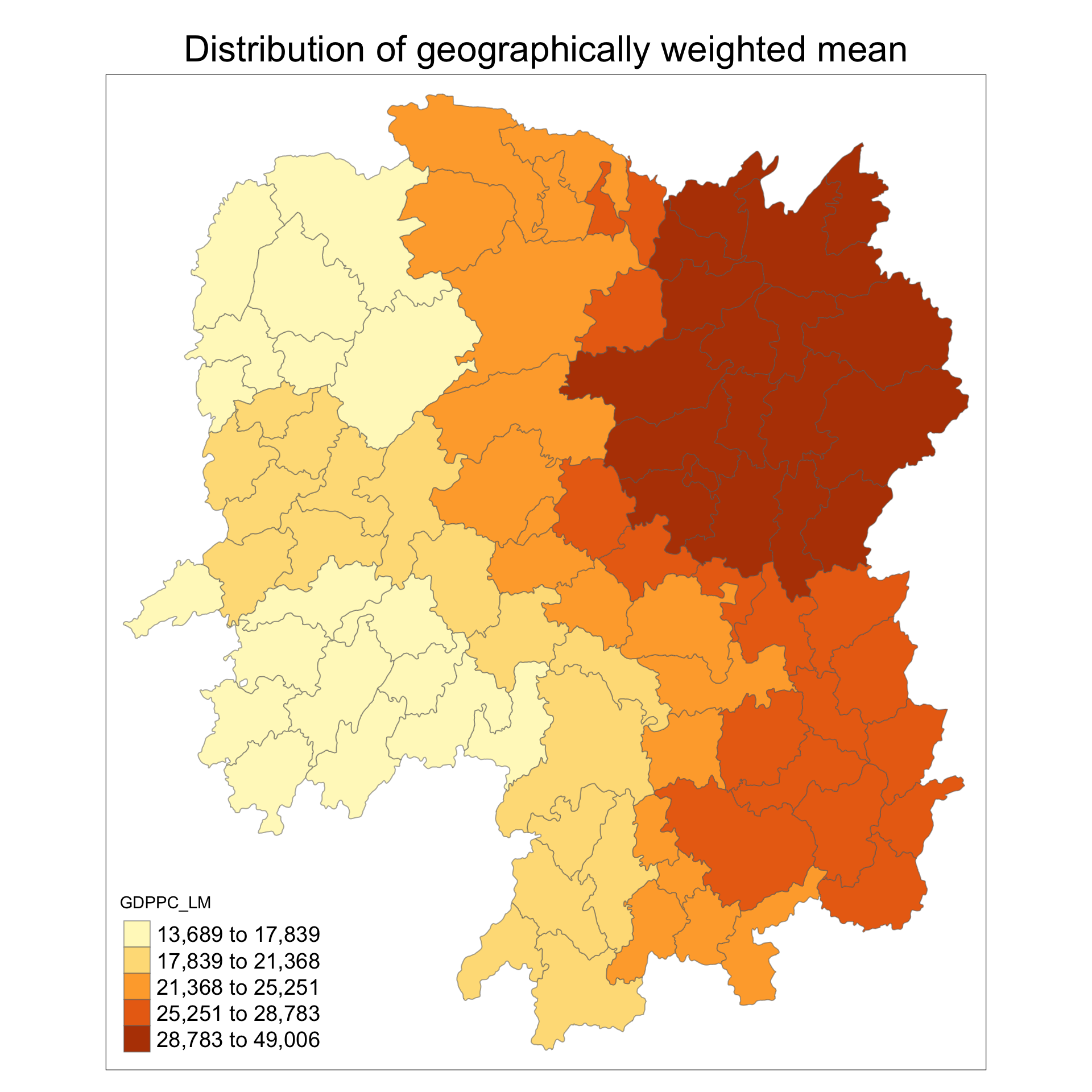
longlat = T)How to interpret the table of the data: GDPPC_LM –> Average of all the neighbours
4.3.2 Preparing the output data
Code chunk below is used to extract SDF data table from gwss object output from gwss(). It will be converted into data.frame. It will be converted into data.frame by using as.data.frame().
Note
Sort or order etc altering functions cannot be applied to the code below, it will mess with the sequence fo the
gstat_df <- as.data.frame(gstat$SDF)Next, cbind() is used to append the newly derived data.frame onto hunan_sf sf data.frame.
hunan_gstat <- cbind(hunan_sf, gstat_df)4.4 Visualising Geographically Weighted Summary Statistics
tm_shape(hunan_gstat)+
  tm_fill("GDPPC_LM",
          n = 5,
          style = "quantile") +
  tm_borders(alpha = 0.5) +
  tm_layout(main.title = "Distribution of geographically weighted mean",
            main.title.position = "center",
            main.title.size = 2.0,
            legend.text.size = 1.2,
            legend.height = 1.5,
            legend.width = 1.5,
            frame = TRUE)