Hands On Exercise 4: Spatio-Temporal Point Patterns Analysis

Author

Georgia Ng

Published

September 10, 2024

Modified

September 13, 2024

4.0 Overview

A spatio-temporal point process (also called space-time or spatial-temporal point process) is a random collection of points, where each point represents the time and location of an event. Examples of events include incidence of disease, sightings or births of a species, or the occurrences of fires, earthquakes, lightning strikes, tsunamis, or volcanic eruptions. In this lesson, you will learn the basic concepts and methods of Spatio-temporal Point Patterns Analysis. You will also gain hands-on experience on using these methods to discover real-world point processes.

The specific questions we would like to answer are:

are the locations of forest fire in Kepulauan Bangka Belitung spatial and spatio-temporally independent?
if the answer is NO, where and when the observed forest fire locations tend to cluster?

4.1 Importing the Packages

For the purpose of this study, five R packages will be used. They are:

rgdal for importing geospatial data in GIS file format such as shapefile into R and save them as Spatial*DataFrame,
maptools for converting Spatial* object into ppp object,
raster for handling raster data in R,
sparr provides functions to estimate fixed and adoptive kernel-smoothed spatial relative risk surfaces via the density-ratio method and perform subsequent inference. Fixed-bandwidth spatiotemporal density and relative risk estimation is also supported.
spatstat for performing Spatial Point Patterns Analysis such as kcross, Lcross, etc., and
tmap for producing cartographic quality thematic maps.

pacman::p_load(sf, raster, spatstat, sparr, tmap, tidyverse)

4.2 The Data

For the purpose of this exercise, two data sets will be used, they are:

forestfires, a csv file provides locations of forest fire detected from the Moderate Resolution Imaging Spectroradiometer (MODIS) sensor data. The data are downloaded from Fire Information for Resource Management System. For the purpose of this exercise, only forest fires within Kepulauan Bangka Belitung will be used.
Kepulauan_Bangka_Belitung, an ESRI shapefile showing the sub-district (i.e. kelurahan) boundary of Kepulauan Bangka Belitung. The data set was downloaded from Indonesia Geospatial portal. The original data covers the whole Indonesia. For the purpose of this exercise, only sub-districts within Kepulauan Bangka Belitung are extracted.

4.2.1 Importing Study Area

kbb <- st_read(dsn="data/rawdata/", 
                   layer="Kepulauan_Bangka_Belitung")

Reading layer `Kepulauan_Bangka_Belitung' from data source 
  `/Users/georgiaxng/georgiaxng/is415-handson/Hands-on_Ex/Hands-on_Ex04/data/rawdata' 
  using driver `ESRI Shapefile'
Simple feature collection with 298 features and 27 fields
Geometry type: POLYGON
Dimension:     XYZ
Bounding box:  xmin: 105.1085 ymin: -3.116593 xmax: 106.8488 ymax: -1.501603
z_range:       zmin: 0 zmax: 0
Geodetic CRS:  WGS 84

Note

Notice that uniquely the polygon in the geometry column when imported is of a Polygon Z type. This means that each polygon not only defines a 2D shape but also includes elevation data with a z-coordinate. This additional z-dimension allows for a more detailed representation of the polygon’s geometry, incorporating vertical information such as elevation or depth.

The below revised code chunk serves to do the following:

Group the boundaries up
Drop the Z values
Transform the coordinate system

kbb_sf <- st_read(dsn="data/rawdata/", 
                   layer="Kepulauan_Bangka_Belitung") %>%
  st_union()%>%
  st_zm(drop = TRUE, what = "ZM")%>%
  st_transform(32748)

Reading layer `Kepulauan_Bangka_Belitung' from data source 
  `/Users/georgiaxng/georgiaxng/is415-handson/Hands-on_Ex/Hands-on_Ex04/data/rawdata' 
  using driver `ESRI Shapefile'
Simple feature collection with 298 features and 27 fields
Geometry type: POLYGON
Dimension:     XYZ
Bounding box:  xmin: 105.1085 ymin: -3.116593 xmax: 106.8488 ymax: -1.501603
z_range:       zmin: 0 zmax: 0
Geodetic CRS:  WGS 84

4.2.2 Converting OWIN

Next, as.owin() is used to convert kbb into an owin object, which is a spatial window or region of interest for point pattern analysis. Once converted to an owin object, we can use it with functions from spatial point pattern analysis packages, such as spatstat, to analyze point patterns within the defined boundary. It helps in setting up the spatial context for further analysis.

kbb_owin <- as.owin(kbb_sf)
kbb_owin

window: polygonal boundary
enclosing rectangle: [512066.8, 705559.4] x [9655398, 9834006] units

Next, class() is used to confirm if the output is indeed an owin object.

class(kbb_owin)

[1] "owin"

4.2.3 Importing and Preparing Forest Fire Data

Next, we will import the forest fire data set into the R environment. The code reads forest fire data from a CSV file, converts it into an sf object using longitude and latitude coordinates, and then reprojects the spatial data from WGS84 to the UTM zone 48S coordinate system. This prepares the data for further spatial analysis in a projection appropriate for the region of interest.

fire_sf <- read_csv("data/rawdata/forestfires.csv") %>%
  st_as_sf(coords = c("longitude", "latitude"),
           crs=4326)%>%
  st_transform(crs = 32748)

Because ppp object only accept numeric or character as mark. The code chunk below is used to convert data type of acq_date to numeric.

fire_sf <- fire_sf %>%
  mutate(DayofYear = yday(acq_date)) %>%
  mutate(Month_num = month(acq_date)) %>%
  mutate(Month_fac = month(acq_date, label= TRUE, abbr = FALSE))

4.3 Visualising The Fire Points

4.3.1 Overall Plot

tm_shape(kbb_sf)+
  tm_polygons() +
tm_shape(fire_sf) +
  tm_dots()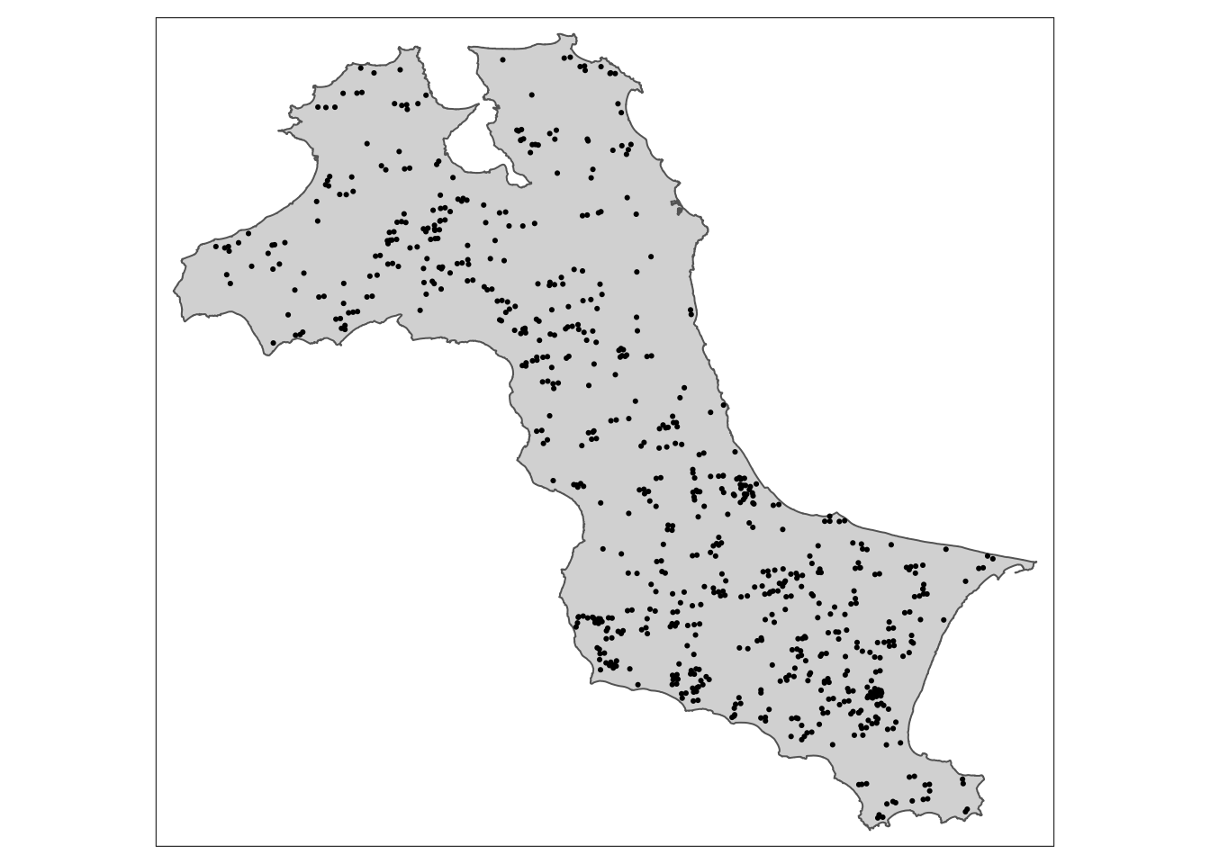

4.3.2 Visualising Geographic Distribution Of Forest Fires By Month

tm_shape(kbb_sf) +
  tm_polygons()+
  tm_shape(fire_sf)+
  tm_dots(size= 0.1)+
  tm_facets(by="Month_fac", free.coords = FALSE, drop.units= TRUE)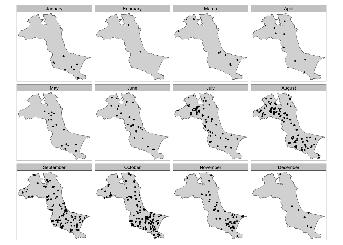

4.4 Computing STKDE by Month

4.4.1 Extracting forest fires by month

The code chunk below is used to remove the unwanted fields from fire_sf sf data.frame. This is because as.ppp() only need the mark field and geometry field from the input sf data frame.

fire_month <- fire_sf %>% 
  select(Month_num)

4.4.2 Creating ppp

The code chunk below is used to derive a ppp object called fire_month from fire_month of data frame.

fire_month_ppp <- as.ppp(fire_month)
fire_month_ppp

Marked planar point pattern: 741 points
marks are numeric, of storage type  'double'
window: rectangle = [521564.1, 695791] x [9658137, 9828767] units

The code chunk below is used to check the output is in the correct object class.

summary(fire_month_ppp)

Marked planar point pattern:  741 points
Average intensity 2.49258e-08 points per square unit

Coordinates are given to 10 decimal places

marks are numeric, of type 'double'
Summary:
   Min. 1st Qu.  Median    Mean 3rd Qu.    Max. 
  1.000   8.000   9.000   8.579  10.000  12.000 

Window: rectangle = [521564.1, 695791] x [9658137, 9828767] units
                    (174200 x 170600 units)
Window area = 29728200000 square units

Next, we will check if there are duplicated point events by using the code chunk below.

any(duplicated(fire_month_ppp))

[1] FALSE

4.4.3 Including Owin Object

The code chunk below is used to combine origin_am_ppp and am_owin objects into one.

fire_month_owin <- fire_month_ppp[kbb_owin]
summary(fire_month_owin)

Marked planar point pattern:  741 points
Average intensity 6.424519e-08 points per square unit

Coordinates are given to 10 decimal places

marks are numeric, of type 'double'
Summary:
   Min. 1st Qu.  Median    Mean 3rd Qu.    Max. 
  1.000   8.000   9.000   8.579  10.000  12.000 

Window: polygonal boundary
2 separate polygons (no holes)
           vertices        area relative.area
polygon 1     47493 11533600000      1.00e+00
polygon 2       256      306427      2.66e-05
enclosing rectangle: [512066.8, 705559.4] x [9655398, 9834006] units
                     (193500 x 178600 units)
Window area = 11533900000 square units
Fraction of frame area: 0.334

plot(fire_month_owin)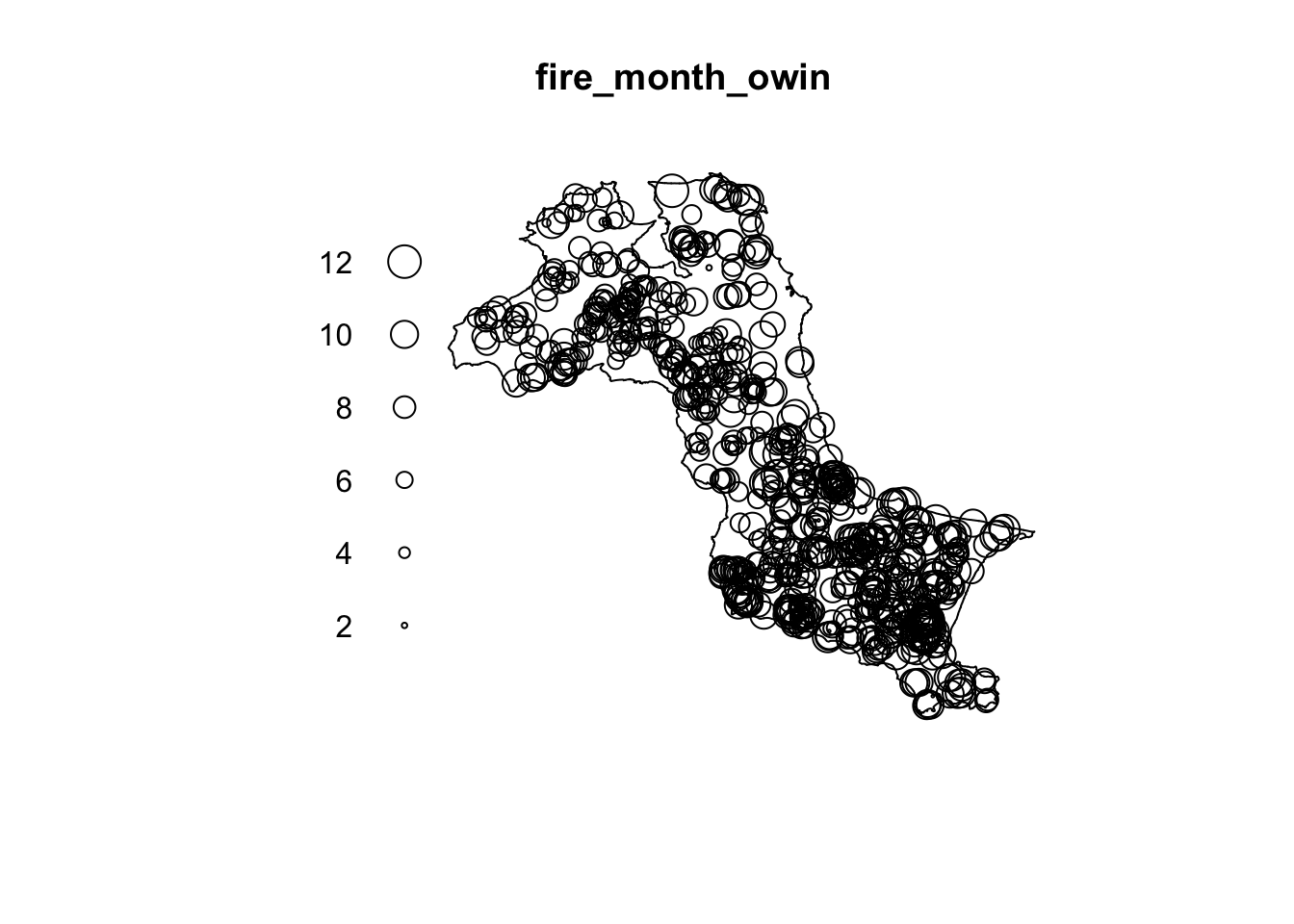

4.4.4 Computing Spatio-Temporal KDE

Next, spattemp.density() of sparr package is used to compute the STKDE.

st_kde <- spattemp.density(fire_month_owin)
summary(st_kde)

Spatiotemporal Kernel Density Estimate

Bandwidths
  h = 15102.47 (spatial)
  lambda = 0.0304 (temporal)

No. of observations
  741 

Spatial bound
  Type: polygonal
  2D enclosure: [512066.8, 705559.4] x [9655398, 9834006]

Temporal bound
  [1, 12]

Evaluation
  128 x 128 x 12 trivariate lattice
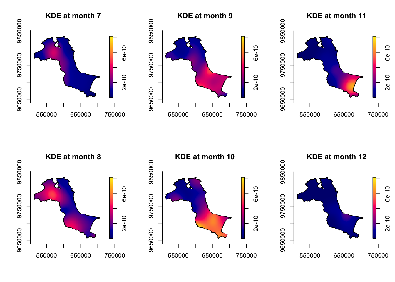
  Density range: [1.233458e-27, 8.202976e-10]

4.4.5 Plotting the spatio-temporal KDE object

In the code chunk below, plot() of R base is used to the KDE for between July 2023 - December 2023.

tims <- c(7,8,9,10,11,12)
par(mfcol=c(2,3))
for(i in tims){ 
  plot(st_kde, i, 
       override.par=FALSE, 
       fix.range=TRUE, 
       main=paste("KDE at month",i))
}

4.5 Computing STKDE by Day of Year

In this section, you will learn how to computer the STKDE of forest fires by day of year.

4.5.1 Creating ppp object

In the code chunk below, DayofYear field is included in the output ppp object.

fire_yday_ppp <- fire_sf %>% 
  select(DayofYear) %>%
  as.ppp()

4.5.2 Including Owin object

Next, code chunk below is used to combine the ppp object and the owin object.

fire_yday_owin <- fire_yday_ppp[kbb_owin]
summary(fire_yday_owin)

Marked planar point pattern:  741 points
Average intensity 6.424519e-08 points per square unit

Coordinates are given to 10 decimal places

marks are numeric, of type 'double'
Summary:
   Min. 1st Qu.  Median    Mean 3rd Qu.    Max. 
   10.0   213.0   258.0   245.9   287.0   352.0 

Window: polygonal boundary
2 separate polygons (no holes)
           vertices        area relative.area
polygon 1     47493 11533600000      1.00e+00
polygon 2       256      306427      2.66e-05
enclosing rectangle: [512066.8, 705559.4] x [9655398, 9834006] units
                     (193500 x 178600 units)
Window area = 11533900000 square units
Fraction of frame area: 0.334

4.5.3

kde_yday <- spattemp.density(
  fire_yday_owin)
summary(kde_yday)

Spatiotemporal Kernel Density Estimate

Bandwidths
  h = 15102.47 (spatial)
  lambda = 6.3198 (temporal)

No. of observations
  741 

Spatial bound
  Type: polygonal
  2D enclosure: [512066.8, 705559.4] x [9655398, 9834006]

Temporal bound
  [10, 352]

Evaluation
  128 x 128 x 343 trivariate lattice
  Density range: [3.959516e-27, 2.751287e-12]

plot(kde_yday)

4.6 Computing STKDE by Day of Year: Improved method

One of the nice function provides in sparr package is BOOT.spattemp(). It support bandwidth selection for standalone spatiotemporal density/intensity based on bootstrap estimation of the MISE, providing an isotropic scalar spatial bandwidth and a scalar temporal bandwidth.

Code chunk below uses BOOT.spattemp() to determine both the spatial bandwidth and the scalar temporal bandwidth.

set.seed(1234)
BOOT.spattemp(fire_yday_owin)

Initialising...Done.
Optimising...
h = 15102.47 ; lambda = 16.84806 
h = 16612.72 ; lambda = 16.84806 
h = 15102.47 ; lambda = 1527.095 
h = 15480.03 ; lambda = 771.9715 
h = 15668.81 ; lambda = 394.4098 
h = 15763.2 ; lambda = 205.6289 
h = 15810.4 ; lambda = 111.2385 
h = 15833.99 ; lambda = 64.04328 
h = 15845.79 ; lambda = 40.44567 
h = 15851.69 ; lambda = 28.64687 
h = 15863.49 ; lambda = 5.049258 
h = 15854.64 ; lambda = 22.74746 
h = 15860.54 ; lambda = 10.94866 
h = 15859.07 ; lambda = 13.89836 
h = 14348.82 ; lambda = 13.89836 
h = 13216.87 ; lambda = 12.42351 
h = 12460.27 ; lambda = 15.37321 
h = 10760.88 ; lambda = 16.11064 
h = 8875.282 ; lambda = 11.68608 
h = 10432.08 ; lambda = 12.97658 
h = 7976.084 ; lambda = 16.66371 
h = 9286.281 ; lambda = 15.60366 
h = 9615.08 ; lambda = 18.73771 
h = 9206.581 ; lambda = 21.61828 
h = 8140.483 ; lambda = 18.23073 
h = 8795.582 ; lambda = 17.70071 
h = 9124.381 ; lambda = 20.83477 
h = 9164.856 ; lambda = 19.52699 
h = 8345.358 ; lambda = 18.48998 
h = 9297.65 ; lambda = 18.67578 
h = 8928.375 ; lambda = 16.8495 
h = 9105.736 ; lambda = 18.85762 
Done.

         h     lambda 
9105.73611   18.85762

4.6.1 Computing spatio-temporal KDE

Now, the STKDE will be derived by using h and lambda values derive in previous step.

kde_yday <- spattemp.density(
  fire_yday_owin,
  h = 9000,
  lambda = 19)
summary(kde_yday)

Spatiotemporal Kernel Density Estimate

Bandwidths
  h = 9000 (spatial)
  lambda = 19 (temporal)

No. of observations
  741 

Spatial bound
  Type: polygonal
  2D enclosure: [512066.8, 705559.4] x [9655398, 9834006]

Temporal bound
  [10, 352]

Evaluation
  128 x 128 x 343 trivariate lattice
  Density range: [2.001642e-19, 2.445724e-12]

4.6.2 Plotting the output spatio-temporal KDE

Last, plot() of sparr package is used to plot the output as shown below.

plot(kde_yday)